Note
Go to the end to download the full example code.
Classify an incomplete vision–language dataset (Oxford‑IIIT Pets) with deep learning
This tutorial demonstrates how to classify samples from an incomplete vision–language dataset using the iMML library. iMML supports robust classification even when some modalities (e.g., text or image) are missing, making it suitable for real‑world multi‑modal data where missingness is common.
We will use the RAGPT algorithm from the iMML classify module on the Oxford‑IIIT Pets dataset
and evaluate its performance.
What you will learn:
How to load a public vision–language dataset (Oxford‑IIIT Pets via Hugging Face Datasets).
How to adapt this workflow to your own vision–language data.
How to train the
RAGPTclassifier when image or text may be missing.How to evaluate the model using cross-validation.
How to visualize predictions.
# sphinx_gallery_thumbnail_number = 1

# License: BSD 3-Clause License
Step 0: Prerequisites
- To run this tutorial, install the extras for deep learning:
pip install imml[deep]
- We also use the Hugging Face Datasets library to load Oxford‑IIIT Pets:
pip install datasets
Step 1: Import required libraries
import shutil
from PIL import Image
from lightning import Trainer
import lightning as L
from matplotlib import pyplot as plt
from torch.utils.data import DataLoader
import torch
import os
import pandas as pd
from sklearn.metrics import matthews_corrcoef, ConfusionMatrixDisplay
from sklearn.preprocessing import LabelEncoder
from datasets import load_dataset
from sklearn.model_selection import StratifiedKFold

from imml.ampute import Amputer
from imml.classify import RAGPT
from imml.load import RAGPTDataset
from imml.model_selection import MMSplitter, train_test_mm_split
from imml.preprocessing import select_complete_samples, select_incomplete_samples
Step 2: Prepare the dataset
We use the oxford-iiit-pet-vl-enriched dataset, a public vision–language dataset with images and captions available on Hugging Face Datasets as visual-layer/oxford-iiit-pet-vl-enriched.
random_state = 42
L.seed_everything(random_state)

# Local working directory (images will be saved here so the method can read paths)
data_folder = "oxford_iiit_pet"
folder_images = os.path.join(data_folder, "imgs")
os.makedirs(folder_images, exist_ok=True)

# Load the dataset
ds = load_dataset("visual-layer/oxford-iiit-pet-vl-enriched", split="train[:70]")

# Build a DataFrame with image paths and captions. We persist images to disk.
n_total = len(ds)
rows = []
for i in range(n_total):
    ex = ds[i]
    img = ex.get("image", None)
    caption = ex.get("caption_enriched", None)
    label = ex.get("label_cat_dog", None)
    img_path = os.path.join(folder_images, f"{i:06d}.jpg")
    try:
        img.save(img_path)
    except Exception:
        img.convert("RGB").save(img_path)
    rows.append({"img": img_path, "text": caption, "label": label})

df = pd.DataFrame(rows)
le = LabelEncoder()
df["class"] = le.fit_transform(df["label"])
Xs = [df[["img"]],df[["text"]]]
y = df["class"]
df["label"].value_counts()
Seed set to 42

label
dog    53
cat    17
Name: count, dtype: int64
Step 3: Simulate missing modalities
To reflect realistic scenarios, we randomly introduce missing data using Amputer. In this case, 60% of training
and test samples will have either text or image missing. You can change this parameter for more or less
amount of incompleteness.
amputer = Amputer(p=0.6, random_state=random_state)
Xs = amputer.fit_transform(Xs)
Step 4: Split the dataset into train and test sets
Split into 40% bank memory, 40% train and 20% test sets.
Xs_train, Xs_test, y_train, y_test = train_test_mm_split(Xs, y, test_size=0.2,
                                                         shuffle=True, stratify=y,
                                                         random_state=random_state)
Xs_train, Xs_bank, y_train, y_bank = train_test_mm_split(Xs_train, y_train, test_size=0.5,
                                                         shuffle=True, stratify=y_train,
                                                         random_state=random_state)

# The bank memory is used to generate retrieval-augmented prompts.
# All samples in the bank need to be complete.
Xs_train_in = select_incomplete_samples(Xs=Xs_bank)
Xs_train = [pd.concat([X, X_in]) for X, X_in in zip(Xs_train, Xs_train_in)]
y_train = pd.concat([y_train, y_bank.loc[Xs_train_in[0].index]])
Xs_bank = select_complete_samples(Xs=Xs_bank)
y_bank = y_bank.loc[Xs_bank[0].index]
print("Xs_train", Xs_train[0].shape)
print("Xs_test", Xs_test[0].shape)
print("Xs_bank", Xs_bank[0].shape)
Xs_train (41, 1)
Xs_test (14, 1)
Xs_bank (15, 1)
Step 5: Training the model
Create the loaders.
modalities = ["image", "text"]
batch_size = 64
n_neighbors = 3

g = torch.Generator()
g.manual_seed(random_state)
train_data = RAGPTDataset(Xs=Xs_train, y=y_train, Xs_bank=Xs_bank, y_bank=y_bank,
                          modalities=modalities, prompt_path=data_folder,
                          n_neighbors=n_neighbors)
train_dataloader = DataLoader(train_data, batch_size=batch_size, shuffle=True, generator=g)

test_data = RAGPTDataset(Xs=Xs_test, y=y_test, mcr=train_data.mcr, modalities=modalities,
                         prompt_path=data_folder, n_neighbors=n_neighbors)
test_dataloader = DataLoader(test_data, batch_size=batch_size, shuffle=False)
Using a slow image processor as `use_fast` is unset and a slow processor was saved with this model. `use_fast=True` will be the default behavior in v4.52, even if the model was saved with a slow processor. This will result in minor differences in outputs. You'll still be able to use a slow processor with `use_fast=False`.
Train the RAGPT model using the generated prompts. For speed in this demo we train for only 2 epochs using
the Lightning library.
GPU available: False, used: False
TPU available: False, using: 0 TPU cores
HPU available: False, using: 0 HPUs

  | Name      | Type             | Params | Mode
-------------------------------------------------------
0 | model     | RAGPTModule      | 118 M  | train
1 | loss_fn   | CrossEntropyLoss | 0      | train
2 | get_probs | Softmax          | 0      | train
-------------------------------------------------------
7.2 M     Trainable params
111 M     Non-trainable params
118 M     Total params
472.956   Total estimated model params size (MB)
21        Modules in train mode
234       Modules in eval mode

Training: |          | 0/? [00:00<?, ?it/s]
Training:   0%|          | 0/1 [00:00<?, ?it/s]
Epoch 0:   0%|          | 0/1 [00:00<?, ?it/s]
Epoch 0: 100%|██████████| 1/1 [00:18<00:00,  0.05it/s]
Epoch 0: 100%|██████████| 1/1 [00:18<00:00,  0.05it/s]
Epoch 0: 100%|██████████| 1/1 [00:18<00:00,  0.05it/s]
Epoch 0:   0%|          | 0/1 [00:00<?, ?it/s]
Epoch 1:   0%|          | 0/1 [00:00<?, ?it/s]
Epoch 1: 100%|██████████| 1/1 [00:18<00:00,  0.06it/s]
Epoch 1: 100%|██████████| 1/1 [00:18<00:00,  0.06it/s]
Epoch 1: 100%|██████████| 1/1 [00:18<00:00,  0.05it/s]`Trainer.fit` stopped: `max_epochs=2` reached.

Epoch 1: 100%|██████████| 1/1 [00:18<00:00,  0.05it/s]
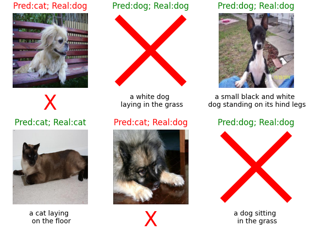
Step 6: Visualize predictions
After training, we can evaluate predictions and visualize the results.
preds = trainer.predict(estimator, test_dataloader)
preds = [pred for batch in preds for pred in batch]
preds = torch.stack(preds).argmax(1).cpu()

nrows, ncols = 2,3
test_df = pd.concat(Xs_test, axis=1)
test_df = pd.concat([test_df, y_test.to_frame("label")], axis=1)
test_df = test_df.reset_index(drop=True)
preds = preds[test_df.index]
fig, axes = plt.subplots(nrows, ncols, constrained_layout=True)
for i, (i_row, row) in enumerate(test_df.sample(n=nrows*ncols, random_state=random_state).iterrows()):
    pred = preds[i_row]
    image_to_show = row["img"]
    caption = row["text"]
    real_class = le.classes_[row["label"]]
    ax = axes[i//ncols, i%ncols]
    ax.axis("off")
    if isinstance(image_to_show, str):
        image_to_show = Image.open(image_to_show).resize((512, 512), Image.Resampling.LANCZOS)
        ax.imshow(image_to_show)
    else:
        ax.plot(0.5, 0.5, 'rx', markersize=100, markeredgewidth=10)
    pred_class = le.classes_[pred]
    c = "green" if pred_class == real_class else "red"
    ax.set_title(f"Pred:{pred_class}; Real:{real_class}", **{"color":c})
    if isinstance(caption, str):
        caption = caption.split(" ")
        if len(caption) >=6:
            caption = caption[:len(caption)//2] + ["\n"] + caption[len(caption)//2:]
            caption = " ".join(caption)
        ax.annotate(caption, xy=(0.5, -0.08), xycoords='axes fraction', ha='center', va='top')
    else:
        ax.annotate("X", xy=(0.5, -0.08), xycoords='axes fraction', ha='center', va='top', color="red", fontsize=30)
Predicting: |          | 0/? [00:00<?, ?it/s]
Predicting:   0%|          | 0/1 [00:00<?, ?it/s]
Predicting DataLoader 0:   0%|          | 0/1 [00:00<?, ?it/s]
Predicting DataLoader 0: 100%|██████████| 1/1 [00:02<00:00,  0.38it/s]
Predicting DataLoader 0: 100%|██████████| 1/1 [00:02<00:00,  0.38it/s]
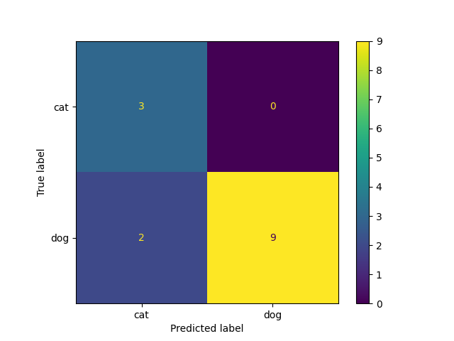
_ = ConfusionMatrixDisplay.from_predictions(y_true=y_test, y_pred=preds,
                                            display_labels=le.classes_)
Step 7: Cross-validation
For robust evaluation, we can use cross-validation. We use a stratified 5-fold cross-validation.
splitter = StratifiedKFold(n_splits=5, shuffle=True, random_state=random_state)
mm_splitter = MMSplitter(splitter=splitter)
performance_list = []
for fold, (Xs_train, Xs_test, y_train, y_test) in enumerate(mm_splitter.split(Xs, y)):
    Xs_train, Xs_bank, y_train, y_bank = train_test_mm_split(Xs_train, y_train, test_size=0.5,
                                                             shuffle=True, stratify=y_train,
                                                             random_state=random_state)
    Xs_train_in = select_incomplete_samples(Xs=Xs_bank)
    Xs_train = [pd.concat([X, X_in]) for X, X_in in zip(Xs_train, Xs_train_in)]
    y_train = pd.concat([y_train, y_bank.loc[Xs_train_in[0].index]])
    Xs_bank = select_complete_samples(Xs=Xs_bank)
    y_bank = y_bank.loc[Xs_bank[0].index]

    g = torch.Generator()
    g.manual_seed(random_state)
    train_data = RAGPTDataset(Xs=Xs_train, y=y_train, Xs_bank=Xs_bank, y_bank=y_bank, modalities=modalities,
                              prompt_path=data_folder, n_neighbors=n_neighbors)
    train_dataloader = DataLoader(train_data, batch_size=batch_size, shuffle=True, generator=g)

    test_data = RAGPTDataset(Xs=Xs_test, y=y_test, mcr=train_data.mcr, modalities=modalities,
                             prompt_path=data_folder, n_neighbors=n_neighbors)
    test_dataloader = DataLoader(test_data, batch_size=batch_size, shuffle=False)

    trainer = Trainer(max_epochs=2, logger=False, enable_checkpointing=False,
                      enable_model_summary=False, enable_progress_bar=False)
    estimator = RAGPT()
    trainer.fit(estimator, train_dataloader)

    preds = trainer.predict(estimator, test_dataloader)
    preds = [pred for batch in preds for pred in batch]
    preds = torch.stack(preds).argmax(1).cpu()

    performance = matthews_corrcoef(y_true=y_test, y_pred=preds)
    performance_list.append(performance)

performance_list = torch.tensor(performance_list)
mean_performance = torch.mean(performance_list)
mean_performance = round(float(mean_performance), 2)
std_performance = torch.std(performance_list)
std_performance = round(float(std_performance), 2)
GPU available: False, used: False
TPU available: False, using: 0 TPU cores
HPU available: False, using: 0 HPUs
`Trainer.fit` stopped: `max_epochs=2` reached.
GPU available: False, used: False
TPU available: False, using: 0 TPU cores
HPU available: False, using: 0 HPUs
`Trainer.fit` stopped: `max_epochs=2` reached.
GPU available: False, used: False
TPU available: False, using: 0 TPU cores
HPU available: False, using: 0 HPUs
`Trainer.fit` stopped: `max_epochs=2` reached.
GPU available: False, used: False
TPU available: False, using: 0 TPU cores
HPU available: False, using: 0 HPUs
`Trainer.fit` stopped: `max_epochs=2` reached.
GPU available: False, used: False
TPU available: False, using: 0 TPU cores
HPU available: False, using: 0 HPUs
`Trainer.fit` stopped: `max_epochs=2` reached.
The performance by fold is:
Fold 1: 0.65
Fold 2: 1.0
Fold 3: 0.78
Fold 4: 1.0
Fold 5: 0.28
The average performance is:
print(f"MCC: {mean_performance} \u00B1 {std_performance}")
MCC: 0.74 ± 0.3
Despite using only 70 instances and minimal training, the performance was very good thanks to the pretrained models.
shutil.rmtree(data_folder, ignore_errors=True)
Summary of results
We trained a model using the RAGPT algorithm available in iMML under 60% randomly missing text and
image modalities. The model demonstrated strong robustness on a cross validation.
This example is intentionally simplified, using only 70 instances for demonstration. For stronger performance and more reliable results, the full dataset and longer training should be used.
Conclusion
This example illustrates how iMML enables state-of-the-art performance in classification, even in the presence of significant modality incompleteness in vision-language datasets.
Total running time of the script: (19 minutes 50.111 seconds)