Survival analysis with incomplete multi-modal data

Survival analysis models time-to-event outcomes, where some samples may be censored because the event was not observed during follow-up. In this tutorial, we show how to use MultiSurv with Lightning to train a small multi-modal survival model.

What you will learn:

• How to represent multi-modal survival data as Xs and y.

• How to wrap the data with MultiSurvDataset and a PyTorch DataLoader.

• How to train MultiSurv with the Lightning Trainer.

• How to obtain survival curves from model predictions.

This tutorial uses a small synthetic dataset so it can run quickly and be adapted to real omics, clinical, imaging, or other multi-modal survival data.

# sphinx_gallery_thumbnail_number = 2

# License: BSD 3-Clause License

Step 1: Import required libraries

import numpy as np
import pandas as pd
import torch
import io
from lightning import Trainer
from scipy.io import arff
from torch.utils.data import DataLoader
import matplotlib.pyplot as plt
import lightning as L
import requests

from imml.ampute import Amputer
from imml.load import MultiSurvDataset
from imml.model_selection import train_test_mm_split
from imml.survival import MultiSurv
from imml.visualize import plot_missing_modality

Step 2: Generate a dataset

Xs is a list of modalities. Each modality has shape (n_samples, n_features_i) and all modalities must be aligned by row. y has two columns: event indicator (where 1 means the event was observed and 0 means the sample was censored) and survival time. We will use the breast cancer dataset (Desmedt, C., Piette, F., Loi et al.) from scikit-survival. For the two modalities, we will use the clinical and gene expression data.

random_state = 42
L.seed_everything(random_state)

data = "https://raw.githubusercontent.com/sebp/scikit-survival/refs/heads/main/sksurv/datasets/data/breast_cancer_GSE7390-metastasis.arff"
data = requests.get(data)
file_object = io.StringIO(data.text)
data, _ = arff.loadarff(file_object)

# 2. Convert to a pandas DataFrame
df = pd.DataFrame(data).rename(columns={"e.tdm": "event", "t.tdm": "time"})
for col in df.select_dtypes([object]).columns:
    df[col] = df[col].str.decode("utf-8")
y = df[["event", "time"]].astype(float)
df = df.drop(columns=y.columns)
clinical = df.drop(columns=df.columns[df.columns.str.endswith("_at")])
clinical = pd.concat([
    clinical.select_dtypes(include="number"),
    pd.get_dummies(clinical.select_dtypes(exclude="number"), drop_first=True).astype(float),
], axis=1)
omics = df[df.columns[df.columns.str.endswith("_at")]]
Xs = [clinical, omics]

print("Samples:", len(Xs[0]), "\t", "Modalities:", len(Xs), "\t", "Features:", [X.shape[1] for X in Xs])
y["event"].value_counts()

Samples: 198     Modalities: 2   Features: [6, 76]

event
0.0    147
1.0     51
Name: count, dtype: int64

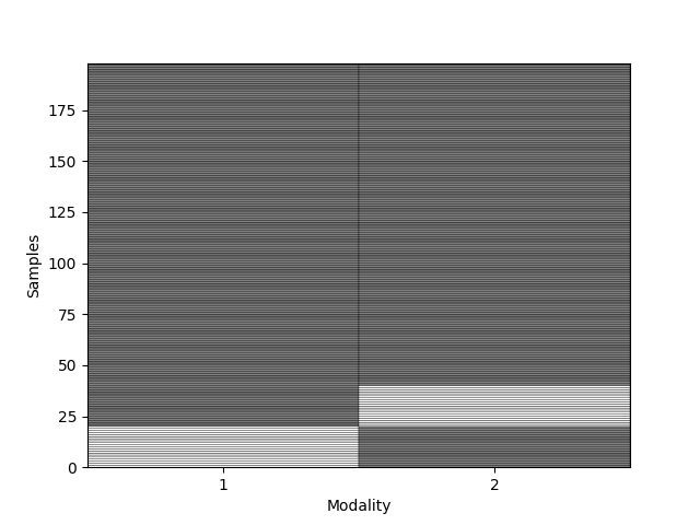
Now, we will introduce some missingness in the data.

amputer = Amputer(p=0.2, random_state=random_state)
Xs = amputer.fit_transform(Xs)
_ = plot_missing_modality(Xs=Xs)

Step 3: Build DataLoaders

We split the dataset into train and test sets.

Xs_train, Xs_test, y_train, y_test = train_test_mm_split(Xs, y, test_size=0.2,
                                                         shuffle=True, stratify=y["event"],
                                                         random_state=random_state)
# ``MultiSurvDataset`` converts pandas and NumPy inputs to tensors and returns batches in the format expected by
# ``MultiSurv``.

train_data = MultiSurvDataset(Xs=Xs_train, y=y_train)
test_data = MultiSurvDataset(Xs=Xs_test, y=y_test)
train_dataloader = DataLoader(train_data, batch_size=12, shuffle=True)
test_dataloader = DataLoader(test_data, batch_size=12, shuffle=False)

Step 4: Train MultiSurv

The default model creates one fully connected extractor per modality. For this small example, we use compact hidden dimensions and only a few time intervals.

model = MultiSurv(input_dim=[X.shape[1] for X in Xs], hidden_dim=16, embed_size=16, t_binds=5)

trainer = Trainer(max_epochs=3, logger=False,
                  enable_checkpointing=False,
                  enable_model_summary=False,
                  enable_progress_bar=False,
)
trainer.fit(model, train_dataloader)

Step 5: Predict survival curves

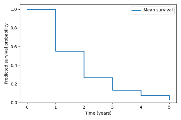
trainer.predict returns one survival matrix per batch. Rows are time points and columns are samples. The first row is fixed to 1 because survival at time zero is 100%.

preds = trainer.predict(model, test_dataloader)
preds = torch.cat(preds, dim=1).detach().cpu().numpy()
time_points_years = model.time_points.detach().cpu().numpy() / 365.0
print("Prediction matrix:", preds.shape)

Prediction matrix: (6, 40)

Step 6: Visualize predictions

Here we plot the average predicted survival curve.

fig, ax = plt.subplots(figsize=(6, 4))
ax.step(time_points_years, preds.mean(axis=1), where="post", label="Mean survival", linewidth=2)
ax.set_xlabel("Time (years)")
ax.set_ylabel("Predicted survival probability")
ax.set_ylim(0, 1.05)
ax.legend()
fig.tight_layout()

Conclusion

This example illustrates how iMML enables multi-modal survival analysis with missing modalities.