Note
Go to the end to download the full example code.
Clustering a multi-modal dataset
Clustering involves grouping samples into distinct groups. In this tutorial, we show how to use iMML to perform clustering on a multi-modal dataset. We also demonstrate how to work with incomplete multi-modal data, where some samples are missing one or more modalities, and how to benchmark the impact of missingness.
What you will learn:
How to represent a dataset with multiple modalities (Xs: list of data matrices).
How to build an iMML pipeline with preprocessing and clustering.
How to evaluate clustering quality with Adjusted Mutual Information (AMI).
How to simulate missing modalities (amputation) and visualize missingness.
How to benchmark robustness against increasing missing-data rates.
This tutorial is fully reproducible and uses a small synthetic dataset. You can easily replace the data-loading section with your own data following the same structure.
# sphinx_gallery_thumbnail_number = 1

# License: BSD 3-Clause License
Step 1: Import required libraries
from sklearn.datasets import make_classification
from sklearn.impute import SimpleImputer
from sklearn.pipeline import make_pipeline
from sklearn.metrics import ConfusionMatrixDisplay, adjusted_mutual_info_score
import numpy as np
import pandas as pd

from imml.preprocessing import MMTransformer, NormalizerNaN
from imml.ampute import Amputer
from imml.cluster import EEIMVC
from imml.visualize import plot_missing_modality
Step 2: Load the dataset
For reproducibility, we generate a small synthetic classification dataset and split the features into two modalities (Xs[0], Xs[1]).
Using your own data:
Represent your dataset as a Python list Xs, one entry per modality.
Each Xs[i] should be a 2D array-like (pandas DataFrame or NumPy array) of shape (n_samples, n_features_i).
All modalities must refer to the same samples and be aligned by row.
random_state = 42
X, y = make_classification(n_samples=50, random_state=random_state, n_clusters_per_class=1, n_classes=3)
X, y = pd.DataFrame(X), pd.Series(y)
# Two modalities: first 10 features and last 10 features
Xs = [X.iloc[:, :10], X.iloc[:, 10:]]
print("Samples:", len(Xs[0]), "\t", "Modalities:", len(Xs), "\t", "Features:", [X.shape[1] for X in Xs])
n_clusters = len(np.unique(y))
y.value_counts()
Samples: 50      Modalities: 2   Features: [10, 10]

0    17
1    17
2    16
Name: count, dtype: int64
Step 3: Clustering
We show how to cluster the multi-modal data using iMML, in this case, using the algorithm EEIMVC. For this
example, we build a pipeline where we first normalize the data and then the samples are clustered.
pipeline = make_pipeline(
    MMTransformer(NormalizerNaN()),
    EEIMVC(n_clusters = n_clusters, random_state=random_state)
)
labels = pipeline.fit_predict(Xs)
Clustering performance is evaluated using the Adjusted Mutual Information (AMI) score, which measures the agreement between predicted clusters and the ground truth, independent of label permutations. We also plot a confusion matrix to visually assess the alignment between predicted clusters and true labels.
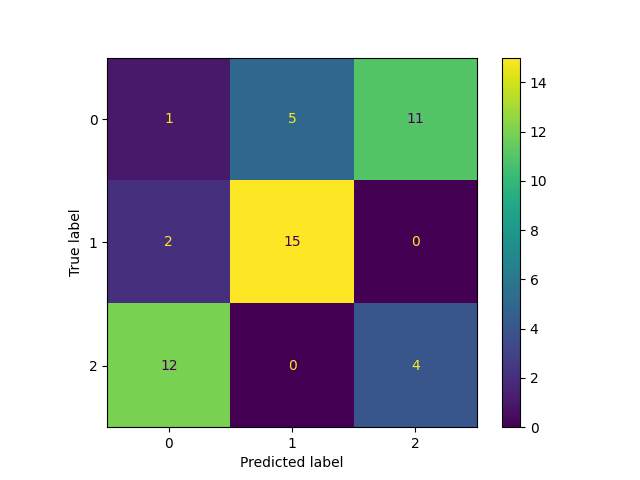
Adjusted Mutual Information Score: 0.2880592167134709
0 20
1 15
2 15
Name: count, dtype: int64
The clustering was quite effective, achieving an AMI score close to 0.5. Note that in clustering, the actual label values are arbitrary, only the grouping structure matters.
Step 4: Simulate missing data (Amputation)
As we mentioned, iMML can be used also for incomplete multi-modal learning, Using Amputer in iMML, we
randomly introduce missing data to simulate a scenario where some modalities are missing. Here, 20% of
the samples will be incomplete.
p = 0.2
amputed_Xs = Amputer(p= p, mechanism="mcar", random_state=42).fit_transform(Xs)
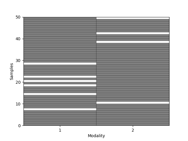
You can visualize which modalities are missing using a binary color map (white for missing modalities, black for available modalities). Each row is a sample; each column is a modality.
_ = plot_missing_modality(Xs=amputed_Xs, sort=False)
Step 5: Clustering with missing data
Now, we repeat the clustering analysis, but this time with the amputed (incomplete) data.
pipeline = make_pipeline(
MMTransformer(NormalizerNaN()),
EEIMVC(n_clusters = n_clusters, random_state=random_state)
)
labels = pipeline.fit_predict(amputed_Xs)
ConfusionMatrixDisplay.from_predictions(y_true=y, y_pred=labels)
print("Adjusted Mutual Information Score:", adjusted_mutual_info_score(labels_true=y, labels_pred=labels))
pd.Series(labels).value_counts()
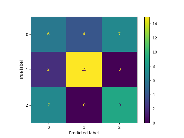
Adjusted Mutual Information Score: 0.35387296796329204

0    19
1    17
2    14
Name: count, dtype: int64
As expected, the clustering performance decreased. However, it remains reasonably good.
Step 6: Benchmarking
We now compare performance with and without missing data. We also include a simple baseline where missing values are first imputed with the feature-wise mean. We repeat the experiments 5 times across increasing missingness to obtain more robust estimates.
ps = np.arange(0., 1., 0.2)
n_times = 5
methods = ["No prior imputation", "Baseline imputation"]
all_metrics = []
for method in methods:
    for p in ps:
        for i in range(n_times):
            pipeline = make_pipeline(
                MMTransformer(NormalizerNaN().set_output(transform="pandas")),
                EEIMVC(n_clusters=n_clusters, random_state=i))
            if method == "Baseline imputation":
                pipeline = make_pipeline(
                    MMTransformer(SimpleImputer().set_output(transform="pandas")),
                    *pipeline)
            pipeline = make_pipeline(Amputer(p=p, mechanism="mcar", random_state=i), *pipeline)
            clusters = pipeline.fit_predict(Xs)
            metric = adjusted_mutual_info_score(labels_true=y, labels_pred=clusters)
            result = {
                "Method": method,
                "Incomplete samples (%)": int(p*100),
                "Iteration": i,
                "AMI": metric,
            }
            all_metrics.append(result)

df = pd.DataFrame(all_metrics)
df = df.sort_values(["Method", "Incomplete samples (%)", "Iteration"], ascending=[True, True, True])
df.head()
g = df.groupby(["Method", "Incomplete samples (%)"])["AMI"]
stats = g.agg(mean="mean", sem=lambda x: x.std(ddof=1) / np.sqrt(len(x))).reset_index()
mean_wide = stats.pivot(index="Incomplete samples (%)", columns="Method", values="mean")
sem_wide  = stats.pivot(index="Incomplete samples (%)", columns="Method", values="sem")
ax = mean_wide.plot(yerr=sem_wide, marker="o", capsize=3, ylabel="Adjusted mutual information")
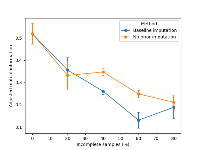
The adjusted mutual information (AMI) indicates how well the clustering aligns with the ground truth.
AMI is 1 when partitions are identical; random partitions have an expected AMI around 0 on average and
can be negative. Here we compare EEIMVC with a simple baseline (feature-wise mean imputation)
across missingness rates from 0% to 80%. We report the mean over 5 repetitions with a
standard-error-of-the-mean (SEM) interval.
Summary of results
Overall, both approaches yield comparable performance at very low and very high missing rates.
When missingness is low, imputations affect only a small fraction of the data, limiting their negative impact.
Conversely, at extremely high missingness, the signal-to-noise ratio deteriorates to the point where both approaches
are similarly constrained by data quality.
With intermediate rates, EEIMVC tends to reach a better clustering performance, highlighting its robustness for
incomplete multi-modal datasets.
Conclusion
This example shows how iMML supports clustering of multi-modal datasets, including scenarios with missing modalities. The pipeline-based design (preprocessing + clustering) and the ability to simulate and visualize missingness make it straightforward to prototype, evaluate, and benchmark real-world multi-modal workflows.
Total running time of the script: (0 minutes 2.601 seconds)