Impute modality- and feature-wise incomplete multi-modal data

When the learning algorithms cannot directly handle missing data, imputation methods become essential to allow their application. Thus, iMML has a module designed for filling missing data, which can be particularly useful when using external methods that are unable to handle missing values directly.

In this tutorial, we will explore how to use iMML to impute an incomplete multi-modal dataset and how to benchmark imputation quality against a simple baseline.

What you will learn:

• How to represent your dataset as Xs (a list of per‑modality matrices).

• How to simulate block‑wise and feature‑wise missingness with Amputer and simple masks.

• How to build an imputation pipeline with StandardScaler + MOFAImputer.

• How to compare MOFAImputer to a baseline mean imputer using Mean Absolute Error (MAE).

• How to visualize missingness before and after imputation.

This tutorial is fully reproducible and uses a small synthetic dataset. You can easily replace the data‑loading section with your own data following the same structure.

# sphinx_gallery_thumbnail_number = 3

# License: BSD 3-Clause License

Step 1: Import required libraries

from sklearn.datasets import make_classification
from sklearn.pipeline import make_pipeline
from sklearn.preprocessing import StandardScaler
from sklearn.impute import SimpleImputer
from sklearn.metrics import mean_absolute_error
import numpy as np
import pandas as pd

from imml.impute import MOFAImputer
from imml.preprocessing import MMTransformer
from imml.ampute import Amputer
from imml.visualize import plot_missing_modality

Step 2: Load the dataset

For reproducibility, we generate a small synthetic classification dataset and split the features into two modalities (Xs[0], Xs[1]).

Using your own data:

• Represent your dataset as a Python list Xs, one entry per modality.

• Each Xs[i] should be a 2D array-like (pandas DataFrame or NumPy array) of shape (n_samples, n_features_i).

• All modalities must refer to the same samples and be aligned by row.

random_state = 42
X, y = make_classification(n_samples=50, random_state=random_state, n_clusters_per_class=1, n_classes=3)
X, y = pd.DataFrame(X), pd.Series(y)
X.columns = X.columns.astype(str)
# Two modalities: first 10 features and last 10 features
Xs = [X.iloc[:, :10], X.iloc[:, 10:]]
names= ["Modality A", "Modality B"]
print("Samples:", len(Xs[0]), "\t", "Modalities:", len(Xs), "\t", "Features:", [X.shape[1] for X in Xs])
n_clusters = len(np.unique(y))
y.value_counts()

Samples: 50      Modalities: 2   Features: [10, 10]

0    17
1    17
2    16
Name: count, dtype: int64

Step 3: Impute missing data

We build an imputation pipeline with two stages: 1) Standardize features per modality (helps MOFA training and makes features comparable). 2) Impute missing modalities with MOFAImputer, which learns shared latent factors across modalities.

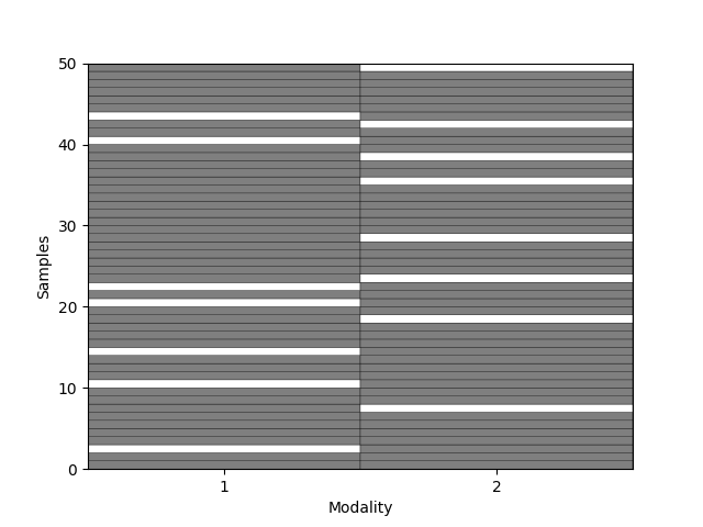
amputed_Xs = Amputer(p= 0.3, mechanism="mcar", random_state=random_state).fit_transform(Xs)

Observe how missing modalities look:

_ = plot_missing_modality(Xs=amputed_Xs, sort=False)

n_components = 4
pipeline = make_pipeline(
    MMTransformer(StandardScaler().set_output(transform="pandas")),
    MOFAImputer(n_components=n_components, random_state=random_state)
)

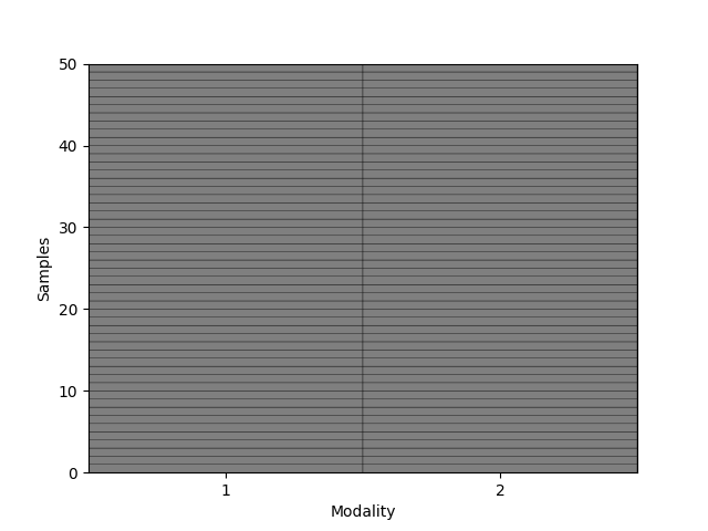
Observe how all modalities are now filled:

imputed_Xs = pipeline.fit_transform(amputed_Xs)
_ = plot_missing_modality(Xs=imputed_Xs, sort=False)

Step 4: Benchmark imputation accuracy

We now compare MOFAImputer with a simple baseline (feature‑wise mean imputation). Design:

• We introduce both modality‑wise (block) and feature‑wise missingness.

• For each missingness rate p, we repeat the procedure 5 times with different seeds.

• We report Mean Absolute Error (MAE) only on entries that were truly missing.

• For MOFAImputer, we standardize before fitting and then invert the scaling to compute MAE in the original space.

ps = np.arange(0.1, 0.8, 0.2)
n_times = 5
methods = ["MOFAImputer", "MeanImputer"]
all_metrics = []

for algorithm in methods:
    for p in ps:
        missing_percentage = int(p*100)
        for i in range(n_times):
            ampute = True
            while ampute: # avoid those iterations where a sample has no available data
                amputed_Xs = Amputer(p=p, random_state=i).fit_transform(Xs)
                for X in amputed_Xs:
                    mask = np.random.default_rng(i).choice([True, False], p= [p,1-p], size = X.shape)
                    X.iloc[mask] = np.nan
                if pd.concat(amputed_Xs, axis=1).isna().all(axis=1).any():
                    i += n_times
                else:
                    ampute = False
            if algorithm == "MeanImputer":
                pipeline = make_pipeline(
                    MMTransformer(SimpleImputer().set_output(transform="pandas"))
                )
            else:
                normalizer = StandardScaler()
                pipeline = make_pipeline(
                    MMTransformer(StandardScaler().set_output(transform="pandas")),
                    MOFAImputer(n_components = n_components, random_state=i))
            masks = [np.isnan(amputed_X) for amputed_X in amputed_Xs]
            imputed_Xs = pipeline.fit_transform(amputed_Xs)
            transformer_list = pipeline[0].transformer_list_
            if algorithm != "MeanImputer":
                imputed_Xs = [pd.DataFrame(transformer.inverse_transform(X), index=X.index, columns=X.columns)
                              for X, transformer in zip(imputed_Xs, transformer_list)]
            metric = np.mean([mean_absolute_error(transformed_X.values[mask], imputed_X.values[mask])
                              for transformed_X,imputed_X,mask in zip(Xs, imputed_Xs, masks)])
            result = {
                "Method": algorithm,
                'Missing rate (%)': int(p*100),
                "Iteration": i,
                "Mean Absolute Error": metric,
            }
            all_metrics.append(result)

df = pd.DataFrame(all_metrics)
df = df.sort_values(["Method", "Missing rate (%)", "Iteration"], ascending=[True, True, True])
df.head()

	Method	Missing rate (%)	Iteration	Mean Absolute Error
0	MOFAImputer	10	0	0.662609
1	MOFAImputer	10	1	0.695769
2	MOFAImputer	10	2	0.725170
3	MOFAImputer	10	3	0.781863
4	MOFAImputer	10	4	0.679923

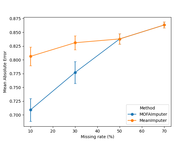
Let's now visualize the results.

g = df.groupby(["Method", "Missing rate (%)"])["Mean Absolute Error"]
stats = g.agg(mean="mean", sem=lambda x: x.std(ddof=1) / np.sqrt(len(x))).reset_index()
mean_wide = stats.pivot(index="Missing rate (%)", columns="Method", values="mean")
sem_wide  = stats.pivot(index="Missing rate (%)", columns="Method", values="sem")
ax = mean_wide.plot(yerr=sem_wide, marker="o", capsize=3, ylabel="Mean Absolute Error")

Summary of results

Across runs and missingness levels, MOFAImputer generally achieves lower MAE than the mean‑imputation baseline at low‑to‑moderate missing rates, reflecting its ability to infer shared latent structure across modalities. As the missing rate becomes very high, both methods degrade and the gap narrows because little signal remains.

Conclusion

Many multi‑modal learning algorithms expect fully observed inputs, making imputation a practical necessity in real‑world workflows. MOFAImputer offers a principled, cross‑modal approach that tends to outperform simple baselines when missingness is not extreme. Thus, ìMML can be used for applying less robuts algorithms to real-world applications.