Note
Go to the end to download the full example code.
Dimensionality reduction: Feature extraction and feature selection
High-dimensional datasets can severely impact machine learning projects, by increasing computational demands, data-adquisition costs and reducing model interpretability. It can also degrade performance due to the curse of dimensionality, as well as the presence of correlated, noisy, or irrelevant features. Consequently, reducing the number of features is often critical. Dimensionality reduction addresses these challenges by enhancing computational efficiency, highlighting key features, reducing noise, and enabling better data visualization.
Dimensionality reduction refers to two main approaches: feature selection and feature extraction.
Feature selection identifies the most relevant features from the dataset.
Feature extraction creates new features by transforming the original ones to capture essential information.
In this tutorial, you will learn how to use JNMF for both feature selection and feature extraction. We will also
cover how to work with missing data, infer modality importance, and visualize the contributions of the top features.
What you will learn:
How to represent your multi-modal dataset as Xs (a list of data matrices).
How to apply
JNMFfor multi-modal feature extraction.How to apply
JNMFFeatureSelectorfor multi-modal feature selection.How to handle missing values.
How to assess modality importance and inspect the selected top features.
How to benchmark different dimensionality-reduction strategies.
# License: BSD 3-Clause License
Step 0: Prerequisites
- To run this tutorial, install the extra dependencies:
pip install imml[r]
Step 1: Import required libraries
from sklearn.impute import SimpleImputer
from sklearn.pipeline import make_pipeline
from sklearn.preprocessing import MinMaxScaler
import pandas as pd
import numpy as np
from sklearn.svm import SVC
from sklearn.preprocessing import FunctionTransformer
from sklearn.metrics import accuracy_score
import matplotlib.patches as mpatches

from imml.decomposition import JNMF
from imml.preprocessing import MMTransformer, ConcatenateMods
from imml.ampute import Amputer
from imml.feature_selection import JNMFFeatureSelector
Step 2: Define plotting functions
def get_modality_importance(Xs, selected_features, weights, names):
    selected_features = {"Feature": selected_features, "Feature Importance": weights}
    selected_features = pd.DataFrame(selected_features)
    selected_features = selected_features.sort_values(by="Feature Importance",
                                                      ascending=False)
    selected_features["Modality"] = selected_features["Feature"].apply(
        lambda x: [name for X,name in zip(Xs, names) if x in X.columns][0])
    selected_features = selected_features.groupby("Modality")["Feature Importance"].sum()
    selected_features = selected_features.div(selected_features.sum()).mul(100)
    selected_features = selected_features.sort_values(ascending=False)
    return selected_features

def get_top_features(Xs, selected_features, weights, components, names):
    selected_features = {"Feature": selected_features, "Feature Importance": weights,
                         "Component": components}
    selected_features = pd.DataFrame(selected_features)
    selected_features = selected_features.sort_values(by="Feature Importance",
                                                      ascending=False)
    selected_features["Modality"] = selected_features["Feature"].apply(
        lambda x: [name for X,name in zip(Xs, names) if x in X.columns][0])
    selected_features["Component"] += 1
    return selected_features

def get_contributions(Xs, selected_features, weights, components, names):
    selected_features = {"Feature": selected_features, "Feature Importance": weights,
                         "Component": components}
    selected_features = pd.DataFrame(selected_features)
    selected_features = selected_features.sort_values(by=["Component", "Feature Importance"],
                                                      ascending=[True, False])
    selected_features["Modality"] = selected_features["Feature"].apply(
        lambda x: [name for X,name in zip(Xs, names) if x in X.columns][0])
    selected_features["Component"] += 1
    return selected_features
Step 3: Load the dataset
We will use the nutrimouse dataset.
Using your own data:
Represent your dataset as a Python list Xs, one entry per modality.
Each Xs[i] should be a 2D array-like (pandas DataFrame or NumPy array) of shape (n_samples, n_features_i).
All modalities must refer to the same samples and be aligned by row.
random_state = 42
Xs = [
    pd.read_csv("https://raw.githubusercontent.com/mvlearn/mvlearn/refs/heads/main/mvlearn/datasets/nutrimouse/gene.csv"),
    pd.read_csv("https://raw.githubusercontent.com/mvlearn/mvlearn/refs/heads/main/mvlearn/datasets/nutrimouse/lipid.csv"),
]
y = pd.read_csv("https://raw.githubusercontent.com/mvlearn/mvlearn/refs/heads/main/mvlearn/datasets/nutrimouse/genotype.csv")
y = y.squeeze()
names= ["Genes", "Lipids"]
print("Samples:", len(Xs[0]), "\t", "Modalities:", len(Xs), "\t", "Features:", [X.shape[1] for X in Xs])
n_clusters = len(np.unique(y))
y.value_counts()
Samples: 40      Modalities: 2   Features: [120, 21]

genotype
wt      20
ppar    20
Name: count, dtype: int64
Step 4: Apply feature selection and feature extraction
n_components = 5
# Feature extraction
pipeline = make_pipeline(MMTransformer(MinMaxScaler().set_output(transform="pandas")),
                         JNMF(n_components=n_components, random_state=random_state))
pipeline.fit(Xs)

# Feature selection
pipeline = make_pipeline(MMTransformer(MinMaxScaler().set_output(transform="pandas")),
                         JNMFFeatureSelector(n_components=n_components, random_state=random_state))
pipeline.fit(Xs)
We can identify and visualize the selected features.
selected_features = get_top_features(Xs=Xs, selected_features= pipeline[-1].selected_features_,
                                     weights= pipeline[-1].weights_, components= pipeline[-1].component_,
                                     names=names)
selected_features
palette = {mod:col for mod, col in zip(names, ["#2ca25f", "#99d8c9"])}
palette_list = [palette[mod] for mod in selected_features["Modality"]]
selected_features = selected_features.assign(color= palette_list).sort_values("Feature Importance")
ax = selected_features.plot(
    kind="barh", x="Feature", y="Feature Importance", legend=False,
    color=selected_features["color"], xlabel="Feature Importance",
    xlim=(0,selected_features["Feature Importance"].max() + .8)
)
ax = ax.legend(handles=[mpatches.Patch(color=color, label=modality) for modality, color in palette.items()],
               loc="lower right")
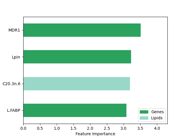
The top features include attributes from both modalities, but the genes seem to be more important overall.
We can visualize the modality relative importance with a barplot.
selected_features = get_modality_importance(
    Xs=Xs, selected_features= pipeline[-1].selected_features_,
    weights= pipeline[-1].weights_, names=names)
selected_features.to_frame()

ax = selected_features.plot(kind= "bar", color= list(palette.values()), ylabel= "Modality Importance (%)", rot=0)
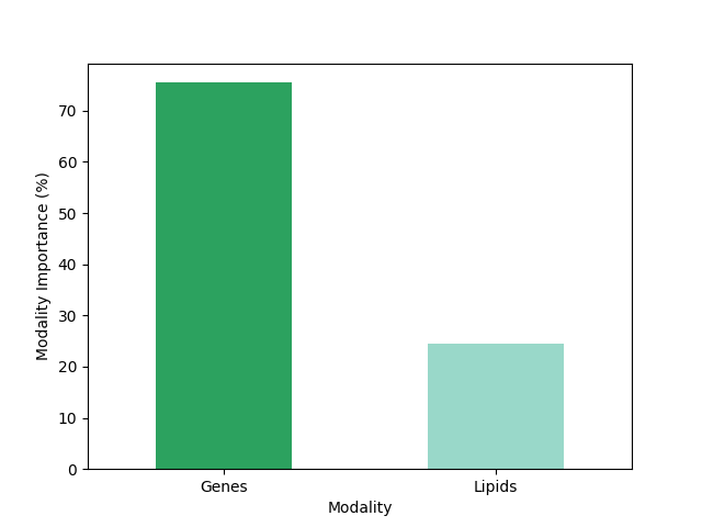
Yes, in fact the genes are the most important modality in this example.
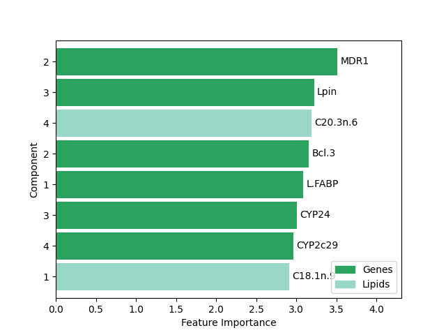
We can also extract features and visualize the original features with the largest contribution to the components.
pipeline = make_pipeline(MMTransformer(MinMaxScaler().set_output(transform="pandas")),
                         JNMFFeatureSelector(n_components = n_components, select_by="component",
                                             random_state=random_state, f_per_component=2))
pipeline.fit(Xs)
selected_features = get_contributions(Xs=Xs, selected_features= pipeline[-1].selected_features_,
                                     weights= pipeline[-1].weights_, components= pipeline[-1].component_,
                                     names= names)
selected_features
palette_list = [palette[mod] for mod in selected_features["Modality"]]
selected_features = selected_features.assign(color= palette_list).sort_values("Feature Importance")
ax = selected_features.plot(
    kind="barh", x="Component", y="Feature Importance", legend=False,
    color=selected_features["color"], xlabel="Feature Importance", width=0.9,
    xlim=(0,selected_features["Feature Importance"].max() + .8)
)
ax.legend(handles=[mpatches.Patch(color=color, label=modality) for modality, color in palette.items()],
          loc="lower right")
ax.bar_label(ax.containers[0], labels=selected_features["Feature"], padding = 3)
[Text(3, 0, 'BACT'), Text(3, 0, 'cHMGCoAS'), Text(3, 0, 'C22.6n.3'), Text(3, 0, 'C22.5n.3'), Text(3, 0, 'L.FABP'), Text(3, 0, 'GK'), Text(3, 0, 'C18.1n.9'), Text(3, 0, 'i.FABP'), Text(3, 0, 'CIDEA'), Text(3, 0, 'SIAT4c')]
Step 6: Analyzing an incomplete multi-modal dataset
We simulated block- and feature-wise missing data. To provide comparative benchmarks, we included baselines using randomly selected features and all available features. The outputs from these methods were then used as inputs for a support vector machine to predict the ground-truth labels. As the feature selection process does not replace missing values, an imputation step was applied prior the classification. We repeat the analysis 5 times with different seeds to have robust results.
ps = np.arange(0., 1., 0.2)
n_times = 5
methods = ["No prior imputation", "Baseline imputation"]
algorithms = ["Feature extraction", "Feature selection", "Randomly selected features", "All features"]
all_metrics = []

for algorithm in algorithms:
    for p in ps:
        for i in range(n_times):
            ampute = True
            while ampute: # avoid those iterations where a sample has no available data
                Xs_train = Amputer(p=p, random_state=i).fit_transform(Xs)
                for X in Xs_train:
                    mask = np.random.default_rng(i).choice([True, False], p= [p,1-p], size = X.shape)
                    X.iloc[mask] = np.nan
                if pd.concat(Xs_train, axis=1).isna().all(axis=1).any():
                    i += n_times
                else:
                    ampute = False
            if algorithm == "Feature extraction":
                pipeline = make_pipeline(
                    MMTransformer(MinMaxScaler().set_output(transform="pandas")),
                    JNMF(n_components = n_components, random_state=i),
                )
            elif algorithm == "Feature selection":
                pipeline = make_pipeline(
                    MMTransformer(MinMaxScaler().set_output(transform="pandas")),
                    JNMFFeatureSelector(n_components = n_components, random_state=i),
                    ConcatenateMods(),
                    SimpleImputer(),
                )
            elif algorithm == "Randomly selected features":
                pipeline = make_pipeline(
                    MMTransformer(MinMaxScaler().set_output(transform="pandas")),
                    ConcatenateMods(),
                    SimpleImputer().set_output(transform="pandas"),
                    FunctionTransformer(lambda x:
                                        x.iloc[:,np.random.default_rng(i).integers(
                                            0, sum([X.shape[1] for X in Xs_train]), size= n_components)]),
                 )
            elif algorithm == "All features":
                pipeline = make_pipeline(
                    MMTransformer(MinMaxScaler().set_output(transform="pandas")),
                    ConcatenateMods(),
                    SimpleImputer().set_output(transform="pandas"),
                 )
            transformed_X = pipeline.fit_transform(Xs_train)
            preds = SVC(random_state=i).fit(transformed_X, y).predict(transformed_X)
            metric = accuracy_score(y_pred=preds, y_true=y)
            result = {
                "Method": algorithm,
                'Missing rate (%)': int(p*100),
                "Iteration": i,
                "Accuracy": metric,
            }
            all_metrics.append(result)

df = pd.DataFrame(all_metrics)
df['Method'] = pd.Categorical(
    df['Method'],
    categories=["Feature extraction", "Feature selection", "All features", "Randomly selected features"],
    ordered=True
)
df = df.sort_values(["Method", "Missing rate (%)", "Iteration"], ascending=[True, True, True])
print(df.shape)
df.head()
(100, 4)
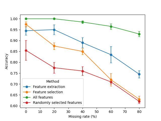
Let's now visualize the results.
g = df.groupby(["Method", "Missing rate (%)"])["Accuracy"]
stats = g.agg(mean="mean", sem=lambda x: x.std(ddof=1) / np.sqrt(len(x))).reset_index()
mean_wide = stats.pivot(index="Missing rate (%)", columns="Method", values="mean")
sem_wide  = stats.pivot(index="Missing rate (%)", columns="Method", values="sem")
ax = mean_wide.plot(yerr=sem_wide, marker="o", capsize=3, ylabel="Accuracy")
Summary of results
Accuracy degrades as the missing‑data rate increases, as a natural consequence of losing information. Using all features achieved always the best performance, a result that was expected. Both dimensionality‑reduction strategies (extraction and selection) perform well when the amount of missing data is not high. Feature extraction with tends to be more robust than feature selection as missingness increases, often yielding the highest accuracy among the reduced representations at moderate-to-high missing rates.
Why feature extraction can be more resilient here:
JNMFlearns low‑rank, shared latent components across modalities, which can attenuate noise introduced by missing values.The selection pipeline requires imputation after selecting features; simple imputers can inject bias, slightly hurting downstream classification in settings with substantial missingness.
Conclusion
In this tutorial we showed how to build compact, informative representations from multi‑modal data and how missingness affects downstream performance.
Overall, iMML provides flexible pipelines to extract or select features across modalities and to benchmark robustness under missing data, helping you choose the right trade‑off between accuracy, efficiency, and interpretability for your application.
Total running time of the script: (0 minutes 2.922 seconds)