Note
Go to the end to download the full example code.
Statistics and interaction structure of a multi-modal dataset
A multi-modal dataset can be characterized beyond basic shape information. With iMML you can:
Summarize core properties of each modality (samples, features, completeness).
Quantify how modalities relate to a target via PID (Partial Information Decomposition): Redundancy (shared info), Uniqueness (modality-specific info), and Synergy (info emerging only when modalities are combined).
What you will learn:
How to compute redundancy, uniqueness, and synergy (PID) with respect to a target using
pid.How to visualize and interpret PID results.
How PID generalizes when you have more than two modalities.
How to describe per‑modality completeness and cross‑modality overlap with
get_summary,plot_summary,plot_combinations, andplot_missing_modality.
This tutorial is fully reproducible and uses a small dataset. You can easily replace the data‑loading section with your own data following the same structure.
# sphinx_gallery_thumbnail_number = 1

# License: BSD 3-Clause License
Step 1: Import required libraries
import pandas as pd

from imml.ampute import Amputer
from imml.statistics import pid
from imml.explore import get_summary
from imml.visualize import plot_pid, plot_summary, plot_combinations, plot_missing_modality
Step 2: Create or load a multi-modal dataset
We will use the nutrimouse dataset.
Using your own data:
Represent your dataset as a Python list Xs, one entry per modality.
Each Xs[i] should be a 2D array-like (pandas DataFrame or NumPy array) of shape (n_samples, n_features_i).
All modalities must refer to the same samples and be aligned by row.
random_state = 42
Xs = [
    pd.read_csv("https://raw.githubusercontent.com/mvlearn/mvlearn/refs/heads/main/mvlearn/datasets/nutrimouse/gene.csv"),
    pd.read_csv("https://raw.githubusercontent.com/mvlearn/mvlearn/refs/heads/main/mvlearn/datasets/nutrimouse/lipid.csv"),
]
y = pd.read_csv("https://raw.githubusercontent.com/mvlearn/mvlearn/refs/heads/main/mvlearn/datasets/nutrimouse/diet.csv")
y = y.squeeze()
mod_names = ["Genes", "Lipids"]

print("Samples:", len(Xs[0]), "\t", "Modalities:", len(Xs), "\t", "Features:", [X.shape[1] for X in Xs])
Samples: 40 Modalities: 2 Features: [120, 21]
Step 3: Compute PID statistics (Redundancy, Uniqueness, Synergy)
Using pid, we quantify the degree of redundancy, uniqueness, and synergy relating input modalities to the target.
With two input modalities, pid returns a dictionary with keys: "Redundancy", "Uniqueness1", "Uniqueness2",
and "Synergy".
rus = pid(Xs=Xs, y=y, random_state=random_state, normalize=True)
rus  # a dict with keys: Redundancy, Uniqueness1, Uniqueness2, Synergy
{'Information': np.float64(1.6094379124341005), 'Redundancy': np.float64(0.7899071869935008), 'Uniqueness1': np.float64(0.0013471577030467743), 'Uniqueness2': np.float64(0.200120459217636), 'Synergy': np.float64(0.008625196085816373)}
Step 4: Visualize the PID as a Venn-like diagram
You can directly pass the rus dict returned by pid to plot_pid. Alternatively, plot_pid can also compute
PID internally if you pass Xs and y, which is convenient when you want a one‑liner.
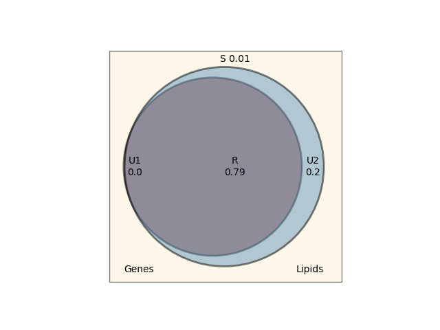
Interpreting PID results
Redundancy: Information about the target available in both modalities. High values suggest overlap.
Uniqueness1/2: Modality‑specific information about the target. High values suggest complementarity.
Synergy: Information that emerges only when modalities are combined. High synergy often indicates interactions.
If redundancy is high while uniqueness and synergy are low, this may suggest that the dataset could be more appropriately analyzed using classical unimodal modeling.
In this case, the redundancy is very high, and the unique information provided by the modality 1 is zero. Therefore, we could just use a classical unimodal learner and, probably, still get the same performance.
Working with more than two modalities
If you have more than two modalities, PID statistics are computed pairwise; pid returns a list of
dictionaries (one per pair). For example, adding a third modality yields three pairwise results.
rus = pid(Xs=Xs + [Xs[0]], y=y, random_state=random_state, normalize=True)
rus
[{'Information': np.float64(1.6094379124341005), 'Redundancy': np.float64(0.7899071869935008), 'Uniqueness1': np.float64(0.0013471577030467743), 'Uniqueness2': np.float64(0.200120459217636), 'Synergy': np.float64(0.008625196085816373)}, {'Information': np.float64(1.2844404775880116), 'Redundancy': np.float64(0.988661991948867), 'Uniqueness1': np.float64(0.0006425105341304864), 'Uniqueness2': np.float64(0.0006425105341452292), 'Synergy': np.float64(0.010052986982857438)}, {'Information': np.float64(1.6094379124341), 'Redundancy': np.float64(0.7899071869162719), 'Uniqueness1': np.float64(0.2001204591932649), 'Uniqueness2': np.float64(0.0013471577176615082), 'Synergy': np.float64(0.008625196172801755)}]
Step 5: Summarize the dataset
Below we first make the dataset a bit more complex by introducing some incomplete samples with Amputer, then
show two views: 1) a dataframe aggregated across modalities (one_row=True) and 2) per‑modality counts (one_row=False).
amputer = Amputer(p=0.6, mechanism="mcar", random_state=random_state)
Xs = amputer.fit_transform(Xs)
The get_summary function provides a compact overview of the multi‑modal dataset.
summary = get_summary(Xs=Xs, one_row=True, compute_pct=True, return_df=True)
summary
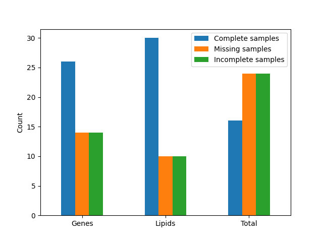
Per‑modality view:
For quick inspection, we can also plot the per‑modality counts. Here we create a bar chart using plot_summary.
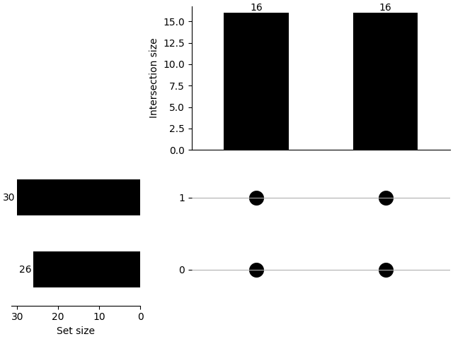
We can also show how is the distribution of the combinations using plot_combinations.
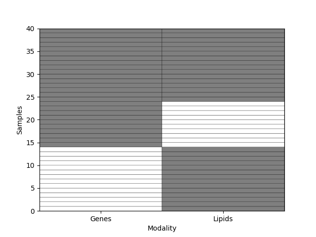
Additionally, we can visualize the missingness pattern using plot_missing_modality.
Conclusion
In this tutorial, we:
Summarized key per‑modality statistics for a multi‑modal dataset.
Quantified redundancy, uniqueness, and synergy with respect to a target using PID.
Visualized and interpreted PID, including the multi‑modality (>2) case.
Explored an incomplete multi-modal dataset with multiple figures.
These insights help you understand complementarity and interactions across modalities, informing model design and feature engineering for downstream multi‑modal learning.
Total running time of the script: (0 minutes 28.472 seconds)