Note
Go to the end to download the full example code.
Modality-wise missing data simulation (Amputation)
Evaluation and benchmarking of new algorithms or models under diverse conditions is essential to ensure their robustness, added value and generalizability. iMML simplifies this process by simulating incomplete multi-modal datasets with modality-wise missing data. This so-called data amputation process allows for controlled testing of methods by introducing missing data from various mechanisms that reflect real-world scenarios where different modalities may be partially observed or entirely missing.
What you will learn:
The four amputation (missingness) mechanisms supported by iMML (PM, MCAR, MNAR, MEM).
How to generate modality-wise incomplete multi-modal datasets with
Amputer.How to visualize missingness patterns across modalities with
plot_missing_modality.How missingness mechanisms and rates affect per-modality data availability.
Missingness mechanisms:
Partial missing (PM): some modalities are fully observed for all samples, while others are partially missing at random.
Missing completely at random (MCAR): missing modalities occur randomly across samples.
Missing not at random (MNAR): certain samples are missing in specific modalities due to factors that influence missingness.
Mutually exclusive missing (MEM): incomplete samples have only one observed modality (an extreme case of MNAR).
This tutorial is fully reproducible and uses a small synthetic dataset. You can easily replace the data-loading section with your own data following the same structure.
# sphinx_gallery_thumbnail_number = 2

# License: BSD 3-Clause License
Step 1: Import required libraries
import numpy as np
import matplotlib.pyplot as plt
import pandas as pd
from IPython.core.display_functions import display

from imml.ampute import Amputer
from imml.explore import get_summary
from imml.visualize import plot_missing_modality, plot_combinations
Step 2: Load the dataset
For illustration, we create a small random multi-modal dataset with 10 samples and 4 modalities.
Using your own data:
Represent your dataset as a Python list Xs, one entry per modality.
Each Xs[i] should be a 2D array-like (pandas DataFrame or NumPy array) of shape (n_samples, n_features_i).
All modalities must refer to the same samples and be aligned by row.
random_state = 7
n_mods = 4
n_samples = 10
rng = np.random.default_rng(random_state)
Xs = [pd.DataFrame(rng.random((n_samples, 10))) for i in range(n_mods)]
Step 3: Simulate missing data
Using Amputer, we introduce missing data to simulate a scenario where some modalities are missing. Here,
80% of the samples will be incomplete following a random missing (MCAR) pattern.
mechanism = "mcar"
p=0.8
amputer = Amputer(mechanism=mechanism, p=p, random_state=random_state)
transformed_Xs = amputer.fit_transform(Xs)
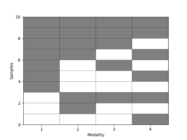
We can visualize which modalities are missing using a binary color map (black = observed, white = missing). Each row is a sample; each column is a modality.
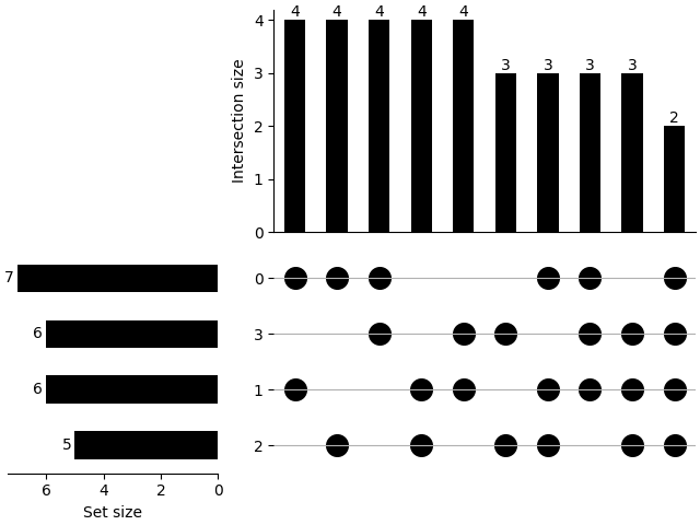
We can also show how is the distribution of the combinations using plot_combinations.
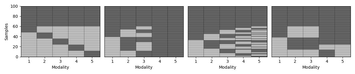
Step 4: Compare amputation mechanisms
We now illustrate the four different amputation patterns: mutually exclusive missing (MEM), partial missing (PM), missing completely at random (MCAR), and missing not at random (MNAR).
mechanism_dict = {"mem": "Mutually exclusive missing",
                  "pm": "Partial missing",
                  "mcar": "Missing completely at random",
                  "mnar": "Missing not at random",
                  }


samples_dict = {}
fig,axs = plt.subplots(1,4, figsize= (12.5,2.5))
for idx, (mechanism, title) in enumerate(mechanism_dict.items()):
    ax = axs[idx]
    transformed_Xs = Amputer(mechanism=mechanism, p=0.8, random_state=random_state).fit_transform(Xs)
    _, ax = plot_missing_modality(Xs=transformed_Xs, ax=ax)
    ax.set_title(title)
    if idx != 0:
        ax.get_yaxis().set_visible(False)
    samples_dict[mechanism_dict[mechanism]] = get_summary(Xs=transformed_Xs, one_row=True)
plt.tight_layout()
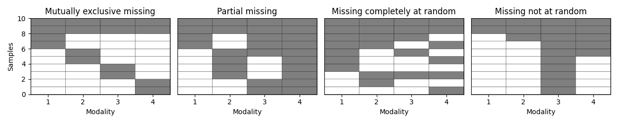
As shown in the table below, all cases have the same numbers of complete and incomplete samples overall. However, the number of observed samples in each modality varies with the missingness pattern.
pd.DataFrame.from_dict(samples_dict, orient= "index")
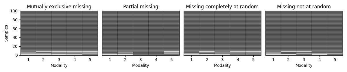
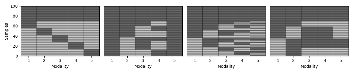
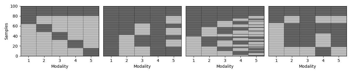
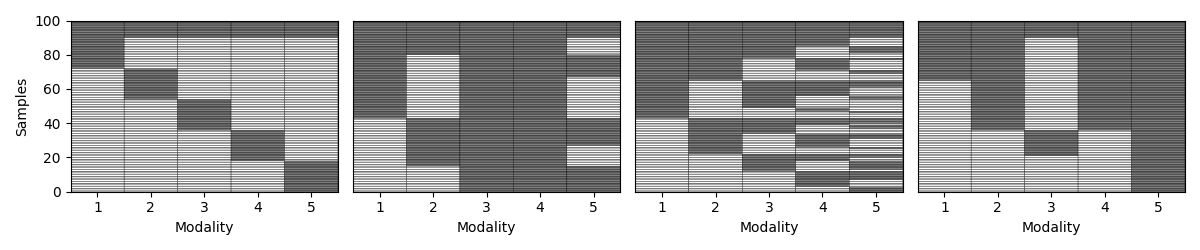
Step 5: Vary the missingness rate
Next, we explore how patterns behave as we increase the percentage of incomplete samples. We amputate a random multi-modal dataset under each mechanism at different missingness rates.
n_mods = 5
n_samples = 100
Xs = [pd.DataFrame(rng.random((n_samples, 10))) for i in range(n_mods)]
for p in np.arange(0.1, 1., 0.1):
    samples_dict = {}
    fig,axs = plt.subplots(1,4, figsize= (12,2.5))
    for idx, (ax, mechanism) in enumerate(zip(axs, list(mechanism_dict.keys()))):
        transformed_Xs = Amputer(mechanism=mechanism, p=p, random_state=random_state+1).fit_transform(Xs)
        _, ax = plot_missing_modality(Xs=transformed_Xs, ax=ax)
        if p == 0.1:
            ax.set_title(mechanism_dict[mechanism])
        if idx != 0:
            ax.get_yaxis().set_visible(False)
        samples_dict[mechanism] = get_summary(Xs=transformed_Xs, one_row=True)
    plt.tight_layout()

    display(pd.DataFrame.from_dict(samples_dict, orient= "index"))
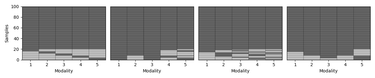
Complete samples Incomplete samples Observed samples per modality Missing samples per modality % Observed samples per modality % Missing samples per modality
mem 90 10 [92, 92, 92, 92, 92] [8, 8, 8, 8, 8] [92, 92, 92, 92, 92] [8, 8, 8, 8, 8]
pm 90 10 [96, 93, 100, 100, 93] [4, 7, 0, 0, 7] [96, 93, 100, 100, 93] [4, 7, 0, 0, 7]
mcar 90 10 [94, 93, 95, 95, 94] [6, 7, 5, 5, 6] [94, 93, 95, 95, 94] [6, 7, 5, 5, 6]
mnar 90 10 [92, 95, 95, 94, 97] [8, 5, 5, 6, 3] [92, 95, 95, 94, 97] [8, 5, 5, 6, 3]
Complete samples Incomplete samples Observed samples per modality Missing samples per modality % Observed samples per modality % Missing samples per modality
mem 80 20 [84, 84, 84, 84, 84] [16, 16, 16, 16, 16] [84, 84, 84, 84, 84] [16, 16, 16, 16, 16]
pm 80 20 [100, 92, 100, 86, 88] [0, 8, 0, 14, 12] [100, 92, 100, 86, 88] [0, 8, 0, 14, 12]
mcar 80 20 [86, 90, 88, 89, 87] [14, 10, 12, 11, 13] [86, 90, 88, 89, 87] [14, 10, 12, 11, 13]
mnar 80 20 [85, 92, 97, 92, 88] [15, 8, 3, 8, 12] [85, 92, 97, 92, 88] [15, 8, 3, 8, 12]
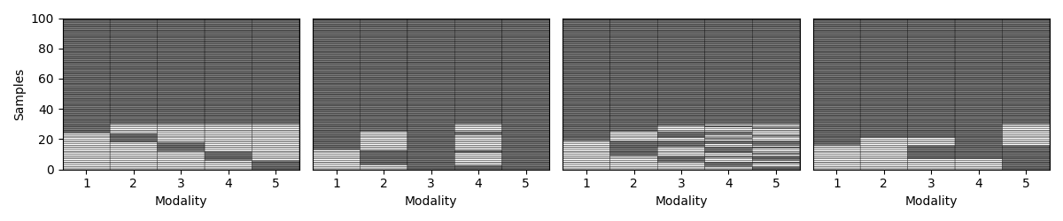
Complete samples Incomplete samples Observed samples per modality Missing samples per modality % Observed samples per modality % Missing samples per modality
mem 70 30 [76, 76, 76, 76, 76] [24, 24, 24, 24, 24] [76, 76, 76, 76, 76] [24, 24, 24, 24, 24]
pm 70 30 [87, 85, 100, 77, 100] [13, 15, 0, 23, 0] [87, 85, 100, 77, 100] [13, 15, 0, 23, 0]
mcar 70 30 [81, 85, 83, 84, 83] [19, 15, 17, 16, 17] [81, 85, 83, 84, 83] [19, 15, 17, 16, 17]
mnar 70 30 [84, 79, 88, 93, 86] [16, 21, 12, 7, 14] [84, 79, 88, 93, 86] [16, 21, 12, 7, 14]
Complete samples Incomplete samples Observed samples per modality Missing samples per modality % Observed samples per modality % Missing samples per modality
mem 60 40 [68, 68, 68, 68, 68] [32, 32, 32, 32, 32] [68, 68, 68, 68, 68] [32, 32, 32, 32, 32]
pm 60 40 [78, 100, 100, 72, 84] [22, 0, 0, 28, 16] [78, 100, 100, 72, 84] [22, 0, 0, 28, 16]
mcar 60 40 [77, 80, 79, 76, 78] [23, 20, 21, 24, 22] [77, 80, 79, 76, 78] [23, 20, 21, 24, 22]
mnar 60 40 [82, 84, 70, 78, 92] [18, 16, 30, 22, 8] [82, 84, 70, 78, 92] [18, 16, 30, 22, 8]
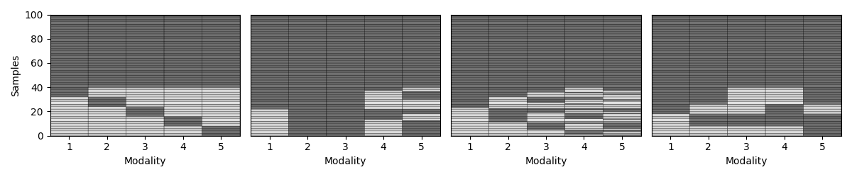
Complete samples Incomplete samples Observed samples per modality Missing samples per modality % Observed samples per modality % Missing samples per modality
mem 50 50 [60, 60, 60, 60, 60] [40, 40, 40, 40, 40] [60, 60, 60, 60, 60] [40, 40, 40, 40, 40]
pm 50 50 [70, 73, 76, 100, 100] [30, 27, 24, 0, 0] [70, 73, 76, 100, 100] [30, 27, 24, 0, 0]
mcar 50 50 [72, 77, 77, 72, 70] [28, 23, 23, 28, 30] [72, 77, 77, 72, 70] [28, 23, 23, 28, 30]
mnar 50 50 [72, 79, 50, 79, 100] [28, 21, 50, 21, 0] [72, 79, 50, 79, 100] [28, 21, 50, 21, 0]
Complete samples Incomplete samples Observed samples per modality Missing samples per modality % Observed samples per modality % Missing samples per modality
mem 40 60 [52, 52, 52, 52, 52] [48, 48, 48, 48, 48] [52, 52, 52, 52, 52] [48, 48, 48, 48, 48]
pm 40 60 [61, 73, 69, 100, 100] [39, 27, 31, 0, 0] [61, 73, 69, 100, 100] [39, 27, 31, 0, 0]
mcar 40 60 [67, 72, 72, 68, 66] [33, 28, 28, 32, 34] [67, 72, 72, 68, 66] [33, 28, 28, 32, 34]
mnar 40 60 [62, 64, 64, 90, 76] [38, 36, 36, 10, 24] [62, 64, 64, 90, 76] [38, 36, 36, 10, 24]
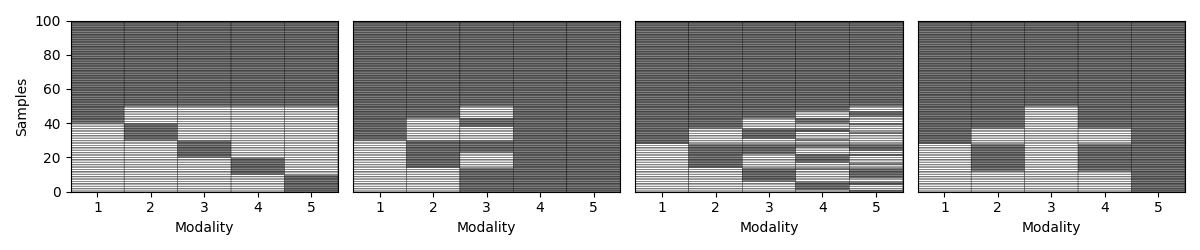
Complete samples Incomplete samples Observed samples per modality Missing samples per modality % Observed samples per modality % Missing samples per modality
mem 30 70 [44, 44, 44, 44, 44] [56, 56, 56, 56, 56] [44, 44, 44, 44, 44] [56, 56, 56, 56, 56]
pm 30 70 [100, 62, 65, 61, 100] [0, 38, 35, 39, 0] [100, 62, 65, 61, 100] [0, 38, 35, 39, 0]
mcar 30 70 [64, 66, 64, 65, 61] [36, 34, 36, 35, 39] [64, 66, 64, 65, 61] [36, 34, 36, 35, 39]
mnar 30 70 [65, 76, 73, 73, 49] [35, 24, 27, 27, 51] [65, 76, 73, 73, 49] [35, 24, 27, 27, 51]
Complete samples Incomplete samples Observed samples per modality Missing samples per modality % Observed samples per modality % Missing samples per modality
mem 20 80 [36, 36, 36, 36, 36] [64, 64, 64, 64, 64] [36, 36, 36, 36, 36] [64, 64, 64, 64, 64]
pm 20 80 [100, 58, 58, 100, 57] [0, 42, 42, 0, 43] [100, 58, 58, 100, 57] [0, 42, 42, 0, 43]
mcar 20 80 [61, 62, 61, 62, 52] [39, 38, 39, 38, 48] [61, 62, 61, 62, 52] [39, 38, 39, 38, 48]
mnar 20 80 [34, 68, 82, 59, 68] [66, 32, 18, 41, 32] [34, 68, 82, 59, 68] [66, 32, 18, 41, 32]
Complete samples Incomplete samples Observed samples per modality Missing samples per modality % Observed samples per modality % Missing samples per modality
mem 10 90 [28, 28, 28, 28, 28] [72, 72, 72, 72, 72] [28, 28, 28, 28, 28] [72, 72, 72, 72, 72]
pm 10 90 [57, 48, 100, 100, 54] [43, 52, 0, 0, 46] [57, 48, 100, 100, 54] [43, 52, 0, 0, 46]
mcar 10 90 [57, 56, 57, 58, 48] [43, 44, 43, 42, 52] [57, 56, 57, 58, 48] [43, 44, 43, 42, 52]
mnar 10 90 [35, 64, 25, 64, 100] [65, 36, 75, 36, 0] [35, 64, 25, 64, 100] [65, 36, 75, 36, 0]
Conclusion
While all the cases have the same number of complete and incomplete samples, each pattern represents a unique distribution of missing data across different modalities, helping researchers to assess the robustness of machine learning models in the presence of incomplete data.
Total running time of the script: (0 minutes 2.988 seconds)